Treemmer: Downsampling massive trees while preserving tree topology

Hello reader, welcome back. It has been a while (school happened), but I'm back with a paper I have been spending time with.

The paper is Treemmer: a tool to reduce large phylogenetic datasets with minimal loss of diversity by Menardo and colleagues, published in BMC Bioinformatics in 2018 [1]. I've also used it on mpox genomes (more on that later). The idea behind Treemmer is simple, and I think that is exactly why it is worth understanding properly.

A few words first

Phylogenetics comes with its own vocabulary, so here are the terms I'll be leaning on.

Term	What it means
Phylogenetic tree	A diagram of how sequences (genomes, genes) are related through shared ancestry.
Leaf (or tip)	One sampled sequence, sitting at the end of a branch. In this post, one leaf is one genome.
Internal node	A point where branches split. It stands for a common ancestor of everything below it.
Branch length	How much genetic change happened along a branch, usually in substitutions per site. Longer branch, more change.
Topology	The branching pattern of the tree: who groups with whom, ignoring branch lengths.
Clade	An ancestor and all of its descendants, i.e. one complete "twig" of the tree.
Redundant	Many leaves that are so similar they add almost no new information.
Polytomy	A node that splits into three or more branches at once, usually because the data can't tell which split came first.
Outgroup	A distant sequence added on purpose so you know where the root of the tree is.

The problem

Public sequence databases keep growing, and if you have ever tried to build a tree from every genome of a pathogen you can download, you already know the pain. The trees get huge, the figures become unreadable, and anything heavier than a quick tree (bootstrapping, molecular clock dating, selection analyses) becomes impractical on a normal computer.

The deeper issue is that these datasets are usually redundant and biased. Nobody coordinated the sampling. Some outbreaks were sequenced hundreds of times, some lineages only a handful of times. So a lot of the leaves in your tree are telling you the same story over and over.

The tools people have used to reduce datasets each have a catch:

• CD-HIT [2] is a classic sequence clustering tool. It groups sequences by percent identity and keeps one representative per group. That works very well for genes and proteins, but it does not scale to whole genomes, and it pays no attention to how the sequences are related evolutionarily. As I understand it, the whole genome problem is twofold. Comparing sequences that are millions of bases long against each other is slow, and closely related genomes are so similar that one identity number is too blunt to separate them: two Mycobacterium tuberculosis genomes from different lineages can still be more than 99.9% identical.
• Tree Pruner [3] works on the tree itself, but you choose the leaves to remove by hand. That is useful for curation, but it is subjective and does not scale to thousands of leaves.
• TreeTrimmer [4] is automatic and phylogeny aware, but it needs you to define operational taxonomic units (OTUs), groupings such as species or genus. For most pathogen datasets those groups either don't exist or are a very rough stand-in for genetic diversity.

Treemmer's pitch is that it needs nothing except a tree with branch lengths.

How Treemmer measures diversity

Treemmer keeps track of diversity with three quantities, all built from branch lengths.

Tree length is the sum of all branch lengths in the tree:

$$L(T) = \sum_{b \in T} \ell_b$$

where $\ell_b$ is the length of branch $b$. A tree carrying more genetic change has a larger $L$.

Relative tree length (RTL) compares what is left after pruning with what you started with:

$$\mathrm{RTL}_k = \frac{L(T_k)}{L(T_0)}$$

$T_0$ is the original tree and $T_k$ is the tree after $k$ rounds of pruning. An RTL of 0.95 means 95% of the original tree length (and so, roughly, of the genetic diversity) is still there.

Patristic distance between two leaves $i$ and $j$ is the sum of the branch lengths along the path connecting them:

$$d(i, j) = \sum_{b \in \mathrm{path}(i,j)} \ell_b$$

where $\mathrm{path}(i,j)$ is the set of branches linking $i$ to $j$ through their most recent common ancestor (MRCA). "Patristic" refers to ancestry: the distance is measured through the ancestor the two leaves share. In the animation below, A and B hang off the same node, so $d(A,B) = 0.05 + 0.07 = 0.12$, while C reaches A through two more branches, giving $d(C,A) = 0.45 + 0.30 + 0.05 = 0.80$.

How the algorithm works

The whole procedure is a loop of two steps.

1. Find neighbours. For every leaf, look for its closest relatives in the tree. First the leaves that hang off the same node (its sisters). If it has none, the leaves two nodes away. Store every pair with its distance $d(i,j)$.
2. Prune. Take the pair with the smallest distance, since those two leaves are the most redundant pair in the tree, and remove one of them at random. Drop every pair that involved the removed leaf.

Repeat until a stopping rule is met. By default Treemmer keeps going until only three leaves remain and records the RTL at every step. You can instead stop at a fixed number of leaves (-X) or when the RTL falls below a threshold (-RTL).

Here it is on a small tree:

Treemmer, step by stepframe 1/18

Leaf labels show each leaf's own (terminal) branch length.

8 leaves · L = 2.54RTL 100.0%

Toy tree with illustrative branch lengths.

Why each cut costs exactly one branch

The round where H is removed shows why Treemmer works so well:

1. H's own branch (0.06) disappears.
2. G is now the only thing hanging off its node, so that node is no longer a split. Treemmer joins G's branch (0.04) to the branch above it (0.20) into a single branch of 0.24. Joining two branches end to end does not change the total length.
3. Nothing else in the tree changes.

So the tree loses exactly the length of the leaf that was removed:

$$L(T_{k+1}) = L(T_k) - \ell_x$$

where $x$ is the leaf removed in round $k+1$ and $\ell_x$ is the length of its terminal branch. In the example, $2.54 - 0.06 = 2.48$.

Now combine that with the pruning rule. The distance between the two leaves of a pair includes both of their own branches, so whichever leaf gets removed, its branch can be no longer than that distance. By always going after the closest pair, Treemmer keeps every cut small. This is a greedy approach: it makes the cheapest-looking choice at each step and never goes back. That does not guarantee the best possible subset at the end, but in practice it behaves very sensibly.

Finding neighbours is the slow part, so the -r (resolution) option lets Treemmer prune several leaves before recalculating the neighbours. It speeds things up a lot, and as you'll see below, it barely changes the result.

What the paper showed

The authors tested Treemmer on two datasets with very different shapes.

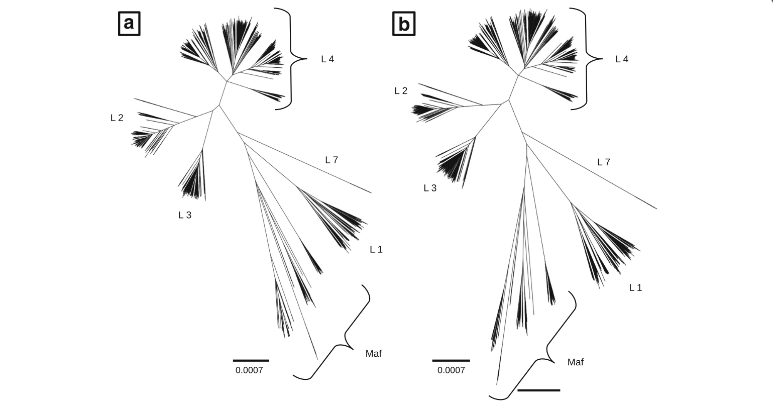
Mycobacterium tuberculosis (MTB). They assembled 10,303 genomes from public Illumina sequencing data after a fairly strict quality control pipeline. Stopping at -RTL 0.95 brought it down to 4,919 leaves. More than half the genomes were dropped, 95% of the tree length was kept, and every lineage was still there.

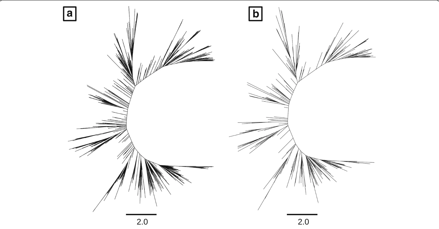
Influenza A (H3N2). A 2,080 sequence tree of the haemagglutinin (HA) gene from Nextstrain. This one is bushy and ladder-like, the typical shape of a virus that keeps replacing itself season after season, and much less redundant. Cutting it down to 250 leaves kept only about 35% of the tree length, but the reduced tree still has the shape of the original.

The most useful comparison is how fast the RTL falls in each dataset as leaves are removed. This curve is called the RTL decay plot, and Treemmer draws it by default. To put both datasets on one axis, the chart below shows the percentage of leaves removed rather than the raw count.

RTL decay, real data from the paper

M. tuberculosisInfluenza A (H3N2)

Show as a table

Leaves removed	M. tuberculosis	Influenza A (H3N2)
25%	99.7%	94.4%
50%	95.9%	79.8%
75%	74.3%	54.0%
90%	43.0%	31.6%

The MTB curve hardly moves until about half of the leaves are gone. That flat start is the signature of a redundant dataset: thousands of genomes can go before you lose any real diversity. The influenza curve starts falling straight away, because almost every leaf carries something unique. So the decay plot is not just a way to choose a size. It is also a quick diagnostic of how redundant your dataset is in the first place.

A few other results worth noting:

• Resolution barely mattered. For MTB, curves with -r set to 1, 10 and 100 were indistinguishable, and 1,000 only drifted late. The authors' rule of thumb is to keep -r about two orders of magnitude (100 times) below the number of leaves, and to compare a few values on a new dataset.
• Molecular clock estimates held up. Trimming the influenza tree to 99%, 90%, 75% and 50% RTL kept the MRCA of the full dataset every time, and the estimated substitution rate and age of the MRCA stayed similar. They recommend protecting outgroups with the metadata option (below) so the root is never pruned.
• Randomness is real but small. Because one leaf of each pair is dropped at random, two runs give slightly different results. Across 100 runs, the largest difference in RTL was about 1% for MTB and about 2.5% for influenza, so it is worth running it a few times.

Trying it on mpox

This is where Treemmer earned its place in my own work. I had a tree of 561 mpox genomes, and like most outbreak datasets it was lopsided. I ran Treemmer with -RTL 0.9, meaning "stop once 10% of the tree length is gone".

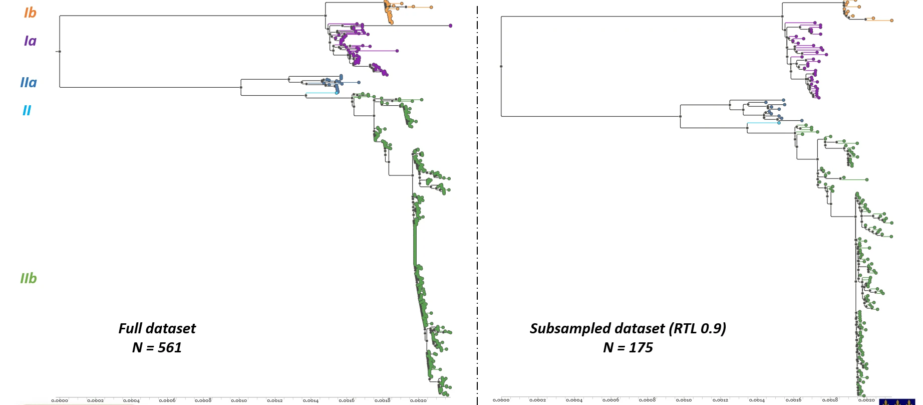
It went from 561 genomes to 175, so about 69% of the genomes were dropped while 90% of the tree length was kept. Every clade (Ia, Ib, IIa, IIb and the single clade II genome) is still there, and the backbone of the tree looks the same. Most of the pruning happened in clade IIb, the long green column on the left. Those are hundreds of near-identical genomes, which is what you would expect given how heavily the 2022 outbreak was sequenced. That is exactly the kind of redundancy Treemmer is built to remove, and the smaller tree is far easier to read and to run heavier analyses on.

The options I'd actually use

Flag	What it does
-X N	Stop when N leaves remain
-RTL x	Stop when RTL falls below x (between 0 and 1)
-r N	Prune N leaves before recalculating neighbours (faster)
-c N	Number of central processing units (CPUs) to use for the neighbour search
-p	Resolve polytomies at random (very large polytomies slow it down)
-lm file	A metadata file of leaf,tag lines, for example country or lineage
-mc N	With -lm, keep at least N leaves for each tag
-lp 0/1/2	Which leaf of the pair to drop: the longer, the shorter, or random (default)
-np	Don't draw the decay plot

The metadata options are what make it practical for surveillance work. You can, for example, make sure every country or every lineage keeps a minimum number of genomes instead of letting the most diverse clade dominate.

A typical run looks like this:

# draw the RTL decay plot for the whole tree
python3 Treemmer_v0.3.py tree.nwk

# keep 90% of tree length, pruning 10 leaves per neighbour search, on 4 CPUs
python3 Treemmer_v0.3.py tree.nwk -RTL 0.9 -r 10 -c 4

The dependencies are ETE3, Joblib, NumPy and Matplotlib, and Treemmer is on Bioconda (conda install -c conda-forge -c bioconda treemmer). If you install with pip, note that ETE3 can fail to build on very recent Python versions (3.13 at the time of writing); a Python 3.11 environment works.

Things to be careful about

The authors are upfront about the limitations, and I think these are the most important part of the paper.

• The output is not a random sample. Diverse clades end up overrepresented compared with how common they really are. If your question depends on frequencies (how common a lineage is, for example), a Treemmer subset is the wrong tool.
• Long branches survive. Poor quality or misaligned sequences tend to produce long branches, and Treemmer will happily keep them. Do your quality control before you trim, not after.
• Rapid expansions get flattened. A recent outbreak or burst of population growth shows up as a big clade of short branches, which is exactly what Treemmer prunes first. You can see this in the mpox tree above. If that expansion is what you are studying, use -lm and -mc to protect it.
• Rebuild the tree afterwards. The trimmed tree from -X or -RTL is for a quick look. For the real analysis, take the genomes that were kept and infer a new tree from them.
• Run it more than once. Results vary a little between runs.

My takeaway

What I like about this paper is how far a very simple idea goes. There is no fancy optimisation, just "find the two most similar things and drop one", repeated with care. The RTL decay plot is the real gem for me, because it turns the vague question "is my dataset redundant?" into a curve you can look at.

If you work with large pathogen datasets and have been picking representative genomes by hand (or by gut feeling), it is worth an afternoon.

Yeah so that's it for this one. If I got something wrong or you have something to add, open an issue on the site's GitHub and let me know.

See you on the next one.

References

1. Menardo F, Loiseau C, Brites D, et al. Treemmer: a tool to reduce large phylogenetic datasets with minimal loss of diversity. BMC Bioinformatics. 2018;19:164. doi:10.1186/s12859-018-2164-8. Code: github.com/fmenardo/Treemmer.
2. Li W, Godzik A. Cd-hit: a fast program for clustering and comparing large sets of protein or nucleotide sequences. Bioinformatics. 2006;22(13):1658-1659. doi:10.1093/bioinformatics/btl158.
3. Krishnamoorthy M, Patel P, Dimitrijevic M, et al. Tree pruner: an efficient tool for selecting data from a biased genetic database. BMC Bioinformatics. 2011;12:51. doi:10.1186/1471-2105-12-51.
4. Maruyama S, Eveleigh RJM, Archibald JM. Treetrimmer: a method for phylogenetic dataset size reduction. BMC Research Notes. 2013;6:145. doi:10.1186/1756-0500-6-145.